Generation Random Numbers on an FPGA
One of the problems with FPGA’s is that you generally have to create a lot of library functions by hand.
For example, random numbers. If you were writing a C program for a microcontoller you would:
#include <stdlib.h>
and then use something like:
int x = rand();
and all the generation stuff is handled in the library for you.
So, how do we generate random numbers on an FPGA and how do we know that they are sufficiently random.
First, we ar going to generate uniform random numbers. How do we prove that the numbers we have generated are sufficiently random.
One fun way is to try and approximate pi by flinging darts randomly at a square. We then imagine a circle that is drawn so that the circles bounds touch the edge of the square (see the diagram below):

If the darts thrown are random enough we can count the number of darts that land within the circle versus the ones outside the circle and use this to approximate pi:
The formula for this is:
area of square:
area of circle:
area of circle / area of square =
Lets first model this in python:
from random import randint
from math import sqrt

circle_count = 0
total_count  = 1000000
for i in range(total_count):
        x = float(randint(0,0x80000000))/(2**31)
        y = float(randint(0,0x80000000))/(2**31)
        hyp = (x**2 + y**2)
        if (hyp<=1):
            circle_count+=1

approx = float(circle_count)/float(total_count)
print str(approx*4.0) + " " + str(circle_count)
So, now we have a method of checking the randomness of our random number generator, lets look a the various options.
1. PRBS For Random Number Generation
The simplest way to generate random numbers is to use a PRBS: http://en.wikipedia.org/wiki/Pseudorandom_binary_sequence
which in hardware is a shift register with some feedback elements:
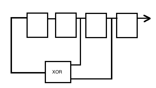
and in verilog looks like:
always @(posedge clk or posedge rst)
    if (rst)
        prbs_out <= 'd2;
    else
        prbs_out <= {prbs_out[29:0], prbs_out[30]^prbs_out[27]};
Firstly its always good to generate a high-level model of what we want to do. Here is some python that allows us to trade off various random number implementations to see how random they are. The python code can be found here (under the python directory):
http://github.com/scottwilson46/FPGARandom
Next, lets write some verilog for one and see how it performs. As you can see from the previous code snippit the implementation of the PRBS itself is fairly simple, but we will see that theres a fair amount of extra work required for the verilog implementation of the maths required to calculate pi. We have to worry about fixed point precision (generally speaking it’s best to keep with fixed point arithmetic for most designs) and also we need to figure out how to do a divide operation in hardware.
For the number representation, since we are generating 31-bit numbers, lets assume that our number representation has: 1-sign bit, 1 integer bit and 29 fractional bits (s1.29)
The first thing we need to do is x^2 and y^2, multiplying a 31-bit number with a 31-bit number will give us a 62-bit number output (s1.60). The best thing to do to stop excessive bit growth through the pipeline is to then convert it back to the original format by losing the bottom 31 bits before performing the add. We can then just look at bit 30 of the add to figure out whether the sum is greater than 1.
Next, we need to calculate the value of pi by dividing the number of times that the sum is less than 1 by the total number of iterations. To do this we need to figure out how to do a divide in hardware. The following page:
http://www.voidware.com/cordic.htm
Has quite a lot of useful information about how to use cordic approximations to calculate a lot of useful mathematical functions, one of which is divide. I create a hardware version of the cordic divide for this purpose. This takes in values of 27-bits and outputs a number in u4.23 format. Multiplying by 4 will convert it to u6.23 format and to get it into a floating point representation we can use:
real pi_real;
pi_real = ($itor(pi_out)) / (2**23);
The entire verilog design and testbench can be found here (under the verilog directory):
http://github.com/scottwilson46/FPGARandom
Simulation
I create a testbench that simply runs the verilog simulation and writes out a .vcd of all the signals in the design.
To run the simulation yourself, you will need to install both icarus verilog and gtkwave:
http://iverilog.icarus.com/home
and
http://gtkwave.sourceforge.net/
You can then use the run script in the verilog directory to set off the simulation (source run_sim).
Timing
I wrote a c-version of the algorithm so that I can accurately time how long it would take to do 1,000,000 iterations of the monte-carlo simulation on a CPU (using the 1.7GHz Intel Core i7 on my Macbook Air).
(C-code on github, here, under the c directory:
http://github.com/scottwilson46/FPGARandom
This gives us around 20ms for the simulation.
For the FPGA version, if we have a clock speed of 100MHz, thats 10ns per calculation (since its all pipelined and after the first value has come out the end of the pipe we get a simulation result every cycle), then we get:
1,000,000 * 10e-9 = 10ms
How fast does it really go?
Without any optimization, quartus reports that the maximum setup failure is 5.57ns, with a clock period of 1ns, giving us 6.67ns as our clock period (around 150MHz).
1,000,000 * 6.67e-9 = 6.67ms
So currently its just over twice as fast, but we can do a number of things to make it faster:
-
We could pipeline the design more (the multipliers are the critical path, we can easily pipeline these).
-
When we make our simulation more complicated (which we will do when we come to look at Black Scholes), the FPGA implementation will still be able to be fully pipelined and give us a value every cycle wheras each iteration of the CPU implementation will be significantly slower.
Next time, we will look at Better random number generators, a hardware version of Mercenne Twister, and hopefully get round to looking at a more complicated monte-carlo simulation of the black-scholes equation.